library(tximport)
library(ggplot2)
library(ggrepel)
library(rhdf5)Class 17: Obtaining and processing SRA datasets on AWS
Class 17 Lab
Q1. What shell command can you use to view the top few lines of your FASTQ file?
head SRR600956.fastqQ2. What length are these sequence reads?
The sequence reads are 38 bases long.
Q3. Can you use the grep command to determine how many total reads are in this file?
grep -c “@SRR600956” SRR600956.fastq
This tells us 25849655 total reads.
Q4. Does your number of reads from grep match the name of the last read in the file? If not why not?
grep -c “@SRR600956” SRR600956.fastq
Yes, the number of reads from the grep matches the name of the last read in the file.
Q5. How would you check that the .fastq files actually look like what we expect for a FASTQ file?
head SRR2156848_1.fastq
Q6. How could you check the number of sequences in each file?
grep -c “^@SRR2156848” SRR2156848_1.fastq
2959900 sequences in each file.
Q7. Check your answer with the bottom of the file using tail and also check the matching mate pair FASTQ file. Do these numbers match? If so why or why not?
tail SRR2156848_1.fastq tail SRR2156848_2.fastq
Yes, these number match.
Q8. Check you have pairs of FASTQ files for all four datasets and that they have the same number of counts in each pair.
ls .fastq grep -c “^@SRR” .fastq
Q9. Fill in the missing kallisto installation/ setup commands
Unzip and untar: tar -zxvf kallisto_linux-v0.44.0.tar.gz
Add kallisto: export PATH=$PATH:/home/ubuntu/kallisto_linux-v0.44.0
Print citation: kallisto cite
Q10. Complete the remianing quantification commands
kallisto quant -i hg19.ensembl -o SRR2156849_quant SRR2156849_1.fastq SRR2156849_2.fastq kallisto quant -i hg19.ensembl -o SRR2156850_quant SRR2156850_1.fastq SRR2156850_2.fastq kallisto quant -i hg19.ensembl -o SRR2156851_quant SRR2156851_1.fastq SRR2156851_2.fastq
Q11. Have a look at the TSV format versions of these files to understand their structure. What do you notice about these fils contents?
These abudnance.tsv files all contain similar structure for each sample. Each file has the same transcript-level quantification results.
Kallisto results:
folders <- dir(pattern = "SRR21568.*_quant$")
samples <- sub("_quant", "", folders)
files <- file.path(folders, "abundance.h5")
names(files) <- samples

files
SRR2156848 SRR2156849
"SRR2156848_quant/abundance.h5" "SRR2156849_quant/abundance.h5"
SRR2156850 SRR2156851
"SRR2156850_quant/abundance.h5" "SRR2156851_quant/abundance.h5" txi.kallisto <- tximport(files, type = "kallisto", txOut = TRUE)1 2 3 4 head(txi.kallisto$counts) SRR2156848 SRR2156849 SRR2156850 SRR2156851
ENST00000539570 0 0 0.00000 0
ENST00000576455 0 0 2.62037 0
ENST00000510508 0 0 0.00000 0
ENST00000474471 0 1 1.00000 0
ENST00000381700 0 0 0.00000 0
ENST00000445946 0 0 0.00000 0Counting summaries:
colSums(txi.kallisto$counts)SRR2156848 SRR2156849 SRR2156850 SRR2156851
2563611 2600800 2372309 2111474 sum(rowSums(txi.kallisto$counts) > 0)[1] 94561Now let’s filter the transcripts:
to.keep <- rowSums(txi.kallisto$counts) > 0
kset.nonzero <- txi.kallisto$counts[to.keep,]

keep2 <- apply(kset.nonzero, 1, sd) > 0
x <- kset.nonzero[keep2,]

dim(x)
[1] 94525 4#PCA
pca <- prcomp(t(x), scale = TRUE)
summary(pca)
Importance of components:
PC1 PC2 PC3 PC4
Standard deviation 183.6379 177.3605 171.3020 1e+00
Proportion of Variance 0.3568 0.3328 0.3104 1e-05
Cumulative Proportion 0.3568 0.6895 1.0000 1e+00##PC1 vs PC2
mycols <- c("blue", "blue", "red", "red")
ggplot(pca$x) +
  aes(PC1, PC2, label = rownames(pca$x)) +
  geom_point(col = mycols) +
  geom_text_repel(col = mycols) +
  theme_bw()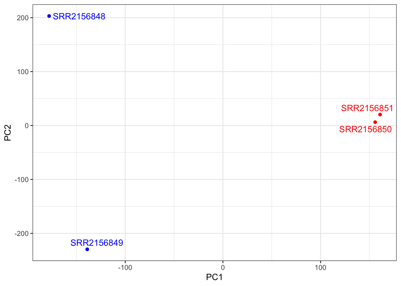
##PC1 vs PC3
ggplot(pca$x) +
  aes(PC1, PC3, label = rownames(pca$x)) +
  geom_point(col = mycols) +
  geom_text_repel(col = mycols) +
  theme_bw()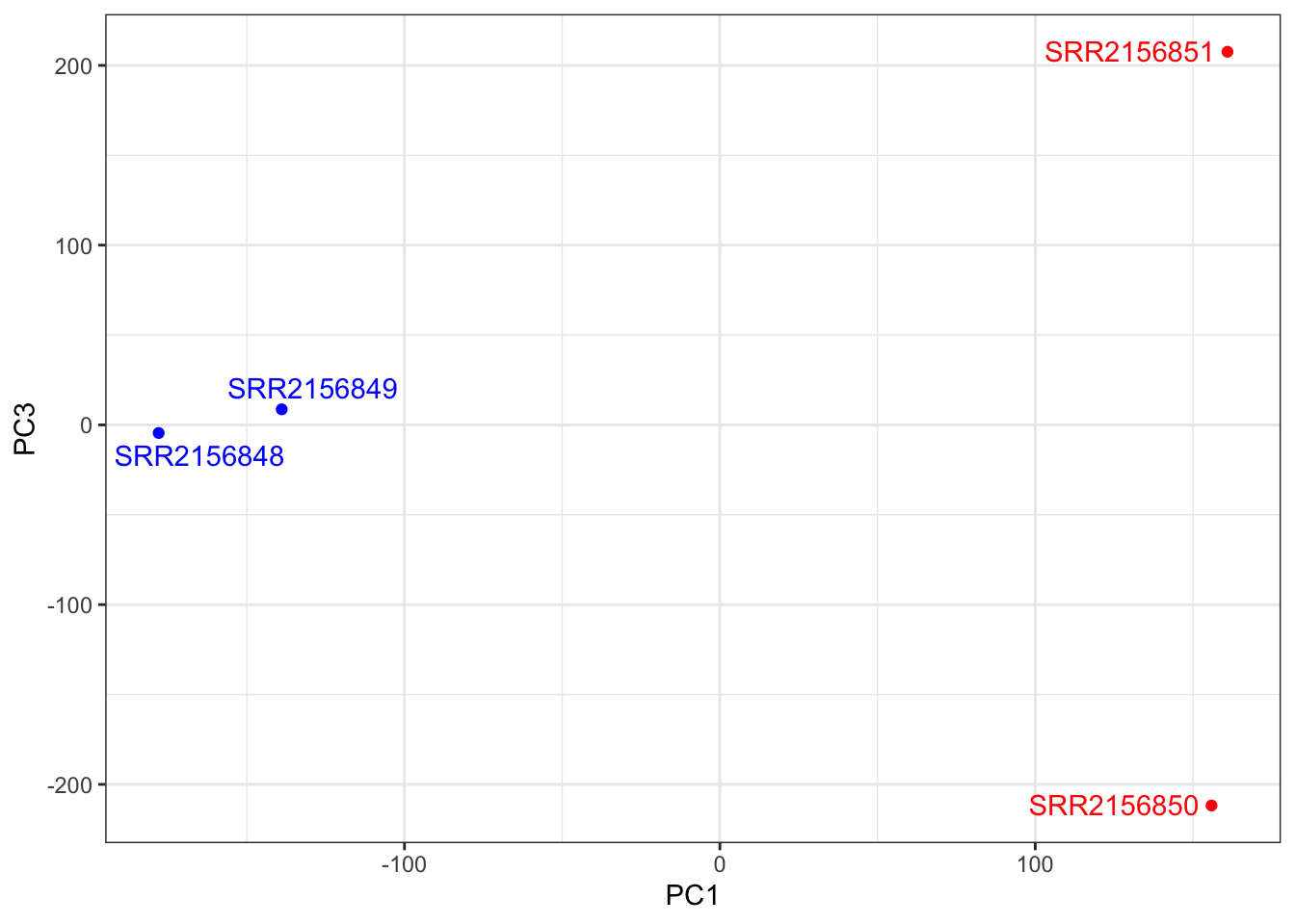
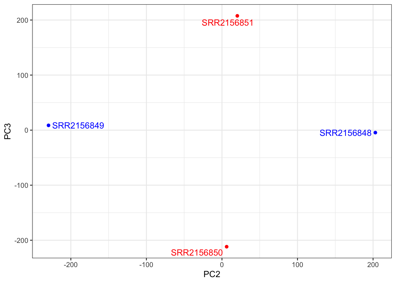
##PC2 vs PC3
ggplot(pca$x) +
  aes(PC2, PC3, label = rownames(pca$x)) +
  geom_point(col = mycols) +
  geom_text_repel(col = mycols) +
  theme_bw()