library(DESeq2)Class 14: RNA-Seq Mini-Project
Background
The data for today’s mini-project comes from a knock-down study of an important HOX gene.
Data Import
colData <- "GSE37704_metadata.csv"
countData <- "GSE37704_featurecounts.csv"
colData = read.csv(colData, row.names = 1)
countData = read.csv(countData, row.names = 1)head(colData) condition
SRR493366 control_sirna
SRR493367 control_sirna
SRR493368 control_sirna
SRR493369 hoxa1_kd
SRR493370 hoxa1_kd
SRR493371 hoxa1_kdhead(countData) length SRR493366 SRR493367 SRR493368 SRR493369 SRR493370
ENSG00000186092 918 0 0 0 0 0
ENSG00000279928 718 0 0 0 0 0
ENSG00000279457 1982 23 28 29 29 28
ENSG00000278566 939 0 0 0 0 0
ENSG00000273547 939 0 0 0 0 0
ENSG00000187634 3214 124 123 205 207 212
SRR493371
ENSG00000186092 0
ENSG00000279928 0
ENSG00000279457 46
ENSG00000278566 0
ENSG00000273547 0
ENSG00000187634 258Clean up (data tidying)
We need to remove that odd first column in countData namely countData$length.
countData$length <- NULL
head(countData)
SRR493366 SRR493367 SRR493368 SRR493369 SRR493370 SRR493371
ENSG00000186092 0 0 0 0 0 0
ENSG00000279928 0 0 0 0 0 0
ENSG00000279457 23 28 29 29 28 46
ENSG00000278566 0 0 0 0 0 0
ENSG00000273547 0 0 0 0 0 0
ENSG00000187634 124 123 205 207 212 258This looks better but there are lots of zero entries in there so let’s get rid of them as we have no data for these.
countData <- countData[rowSums(countData) > 0, ]DESeq Analysis
Setting up the required DESeq object
countData <- as.matrix(countData)

all(colnames(countData) == rownames(colData))
[1] TRUEcolData <- colData[colnames(countData), , drop = FALSE]
all(colnames(countData) == rownames(colData))[1] TRUERunning DESeq
dds <- DESeqDataSetFromMatrix(
  countData = countData,
  colData = colData,
  design = ~ condition
)
Warning in DESeqDataSet(se, design = design, ignoreRank): some variables in
design formula are characters, converting to factorsdds$condition <- relevel(dds$condition, "control_sirna")
dds <- DESeq(dds)estimating size factorsestimating dispersionsgene-wise dispersion estimatesmean-dispersion relationshipfinal dispersion estimatesfitting model and testingGetting results
res <- results(dds)
summary(res)
out of 15975 with nonzero total read count
adjusted p-value < 0.1
LFC > 0 (up)       : 4349, 27%
LFC < 0 (down)     : 4396, 28%
outliers [1]       : 0, 0%
low counts [2]     : 1237, 7.7%
(mean count < 0)
[1] see 'cooksCutoff' argument of ?results
[2] see 'independentFiltering' argument of ?resultsres[order(res$padj), ][1:10, ]log2 fold change (MLE): condition hoxa1 kd vs control sirna
Wald test p-value: condition hoxa1 kd vs control sirna
DataFrame with 10 rows and 6 columns
baseMean log2FoldChange lfcSE stat pvalue
<numeric> <numeric> <numeric> <numeric> <numeric>
ENSG00000117519 4483.63 -2.42272 0.0600016 -40.3776 0
ENSG00000183508 2053.88 3.20196 0.0724172 44.2154 0
ENSG00000159176 5692.46 -2.31374 0.0575534 -40.2016 0
ENSG00000116016 4423.95 -1.88802 0.0431680 -43.7366 0
ENSG00000164251 2348.77 3.34451 0.0690718 48.4208 0
ENSG00000124766 2576.65 2.39229 0.0617086 38.7675 0
ENSG00000124762 28106.12 1.83226 0.0388966 47.1058 0
ENSG00000106366 43719.13 -1.84405 0.0419165 -43.9933 0
ENSG00000188153 2944.13 2.26608 0.0552681 41.0016 0
ENSG00000122861 28007.14 2.26253 0.0552183 40.9742 0
padj
<numeric>
ENSG00000117519 0
ENSG00000183508 0
ENSG00000159176 0
ENSG00000116016 0
ENSG00000164251 0
ENSG00000124766 0
ENSG00000124762 0
ENSG00000106366 0
ENSG00000188153 0
ENSG00000122861 0Volcano Plot
library(ggplot2)

res_df <- as.data.frame(res)
res_df$padj[is.na(res_df$padj)] <- 1
res_df$padj_plot <- pmax(res_df$padj, 1e-300)

mycols <- rep("gray", nrow(res_df))
mycols[abs(res_df$log2FoldChange) > 2] <- "blue"
mycols[res_df$padj > 0.01] <- "gray"

ggplot(res_df) +
  aes(x = log2FoldChange, y = -log10(padj_plot)) +
  geom_point(col = mycols) +
  xlab("Log2(FoldChange)") +
  ylab("-Log10(Adj P-value)") +
  geom_vline(xintercept = c(-2, 2)) +
  geom_hline(yintercept = -log10(0.01))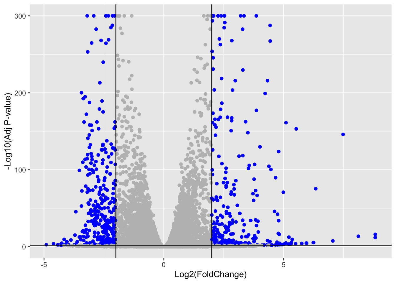
Add Annotation
library("AnnotationDbi")
library("org.Hs.eg.db")columns(org.Hs.eg.db) [1] "ACCNUM" "ALIAS" "ENSEMBL" "ENSEMBLPROT" "ENSEMBLTRANS"
[6] "ENTREZID" "ENZYME" "EVIDENCE" "EVIDENCEALL" "GENENAME"
[11] "GENETYPE" "GO" "GOALL" "IPI" "MAP"
[16] "OMIM" "ONTOLOGY" "ONTOLOGYALL" "PATH" "PFAM"
[21] "PMID" "PROSITE" "REFSEQ" "SYMBOL" "UCSCKG"
[26] "UNIPROT" res$symbol = mapIds(org.Hs.eg.db,
keys = rownames(res),
keytype = "ENSEMBL",
column = "SYMBOL",
multiVals = "first")'select()' returned 1:many mapping between keys and columnsres$entrez = mapIds(org.Hs.eg.db,
keys = row.names(res),
keytype = "ENSEMBL",
column = "ENTREZID",
multiVals = "first")'select()' returned 1:many mapping between keys and columnsres$name = mapIds(org.Hs.eg.db,
keys = row.names(res),
keytype = "ENSEMBL",
column = "GENENAME",
multiVals = "first")'select()' returned 1:many mapping between keys and columnshead(res, 10)log2 fold change (MLE): condition hoxa1 kd vs control sirna
Wald test p-value: condition hoxa1 kd vs control sirna
DataFrame with 10 rows and 9 columns
baseMean log2FoldChange lfcSE stat pvalue
<numeric> <numeric> <numeric> <numeric> <numeric>
ENSG00000279457 29.913579 0.1792571 0.3248216 0.551863 5.81042e-01
ENSG00000187634 183.229650 0.4264571 0.1402658 3.040350 2.36304e-03
ENSG00000188976 1651.188076 -0.6927205 0.0548465 -12.630158 1.43990e-36
ENSG00000187961 209.637938 0.7297556 0.1318599 5.534326 3.12428e-08
ENSG00000187583 47.255123 0.0405765 0.2718928 0.149237 8.81366e-01
ENSG00000187642 11.979750 0.5428105 0.5215598 1.040744 2.97994e-01
ENSG00000188290 108.922128 2.0570638 0.1969053 10.446970 1.51282e-25
ENSG00000187608 350.716868 0.2573837 0.1027266 2.505522 1.22271e-02
ENSG00000188157 9128.439422 0.3899088 0.0467163 8.346304 7.04321e-17
ENSG00000237330 0.158192 0.7859552 4.0804729 0.192614 8.47261e-01
padj symbol entrez name
<numeric> <character> <character> <character>
ENSG00000279457 6.86555e-01 NA NA NA
ENSG00000187634 5.15718e-03 SAMD11 148398 sterile alpha motif ..
ENSG00000188976 1.76549e-35 NOC2L 26155 NOC2 like nucleolar ..
ENSG00000187961 1.13413e-07 KLHL17 339451 kelch like family me..
ENSG00000187583 9.19031e-01 PLEKHN1 84069 pleckstrin homology ..
ENSG00000187642 4.03379e-01 PERM1 84808 PPARGC1 and ESRR ind..
ENSG00000188290 1.30538e-24 HES4 57801 hes family bHLH tran..
ENSG00000187608 2.37452e-02 ISG15 9636 ISG15 ubiquitin like..
ENSG00000188157 4.21963e-16 AGRN 375790 agrin
ENSG00000237330 NA RNF223 401934 ring finger protein ..Let’s reorder these results by adjusted p-value and save them to a CSV file in our current project directory.
res <- res[!is.na(res$padj), ]
res <- res[order(res$padj), ]
write.csv(as.data.frame(res), file = "deseq_results.csv")
Pathway Analysis
Let’s load the packages and setup the KEGG data-sets we need:
library(pathview)##############################################################################
Pathview is an open source software package distributed under GNU General
Public License version 3 (GPLv3). Details of GPLv3 is available at
http://www.gnu.org/licenses/gpl-3.0.html. Particullary, users are required to
formally cite the original Pathview paper (not just mention it) in publications
or products. For details, do citation("pathview") within R.
The pathview downloads and uses KEGG data. Non-academic uses may require a KEGG
license agreement (details at http://www.kegg.jp/kegg/legal.html).
##############################################################################library(gage)library(gageData)
data(kegg.sets.hs)
data(sigmet.idx.hs)
kegg.sets.hs = kegg.sets.hs[sigmet.idx.hs]
head(kegg.sets.hs, 3)$`hsa00232 Caffeine metabolism`
[1] "10" "1544" "1548" "1549" "1553" "7498" "9"
$`hsa00983 Drug metabolism - other enzymes`
[1] "10" "1066" "10720" "10941" "151531" "1548" "1549" "1551"
[9] "1553" "1576" "1577" "1806" "1807" "1890" "221223" "2990"
[17] "3251" "3614" "3615" "3704" "51733" "54490" "54575" "54576"
[25] "54577" "54578" "54579" "54600" "54657" "54658" "54659" "54963"
[33] "574537" "64816" "7083" "7084" "7172" "7363" "7364" "7365"
[41] "7366" "7367" "7371" "7372" "7378" "7498" "79799" "83549"
[49] "8824" "8833" "9" "978"
$`hsa00230 Purine metabolism`
[1] "100" "10201" "10606" "10621" "10622" "10623" "107" "10714"
[9] "108" "10846" "109" "111" "11128" "11164" "112" "113"
[17] "114" "115" "122481" "122622" "124583" "132" "158" "159"
[25] "1633" "171568" "1716" "196883" "203" "204" "205" "221823"
[33] "2272" "22978" "23649" "246721" "25885" "2618" "26289" "270"
[41] "271" "27115" "272" "2766" "2977" "2982" "2983" "2984"
[49] "2986" "2987" "29922" "3000" "30833" "30834" "318" "3251"
[57] "353" "3614" "3615" "3704" "377841" "471" "4830" "4831"
[65] "4832" "4833" "4860" "4881" "4882" "4907" "50484" "50940"
[73] "51082" "51251" "51292" "5136" "5137" "5138" "5139" "5140"
[81] "5141" "5142" "5143" "5144" "5145" "5146" "5147" "5148"
[89] "5149" "5150" "5151" "5152" "5153" "5158" "5167" "5169"
[97] "51728" "5198" "5236" "5313" "5315" "53343" "54107" "5422"
[105] "5424" "5425" "5426" "5427" "5430" "5431" "5432" "5433"
[113] "5434" "5435" "5436" "5437" "5438" "5439" "5440" "5441"
[121] "5471" "548644" "55276" "5557" "5558" "55703" "55811" "55821"
[129] "5631" "5634" "56655" "56953" "56985" "57804" "58497" "6240"
[137] "6241" "64425" "646625" "654364" "661" "7498" "8382" "84172"
[145] "84265" "84284" "84618" "8622" "8654" "87178" "8833" "9060"
[153] "9061" "93034" "953" "9533" "954" "955" "956" "957"
[161] "9583" "9615" foldchanges <- res$log2FoldChange
names(foldchanges) <- res$entrez
foldchanges <- foldchanges[!is.na(names(foldchanges))]
foldchanges <- foldchanges[!is.na(foldchanges)]
head(foldchanges) 1266 54855 1465 2034 2150 6659
-2.422719 3.201955 -2.313738 -1.888019 3.344508 2.392288 Let’s run KEGG pathway enrichment with gage
keggres <- gage(foldchanges, gsets = kegg.sets.hs)Let’s take a peek at the top pathways
head(keggres$greater) p.geomean stat.mean p.val
hsa00140 Steroid hormone biosynthesis 0.002628156 2.958807 0.002628156
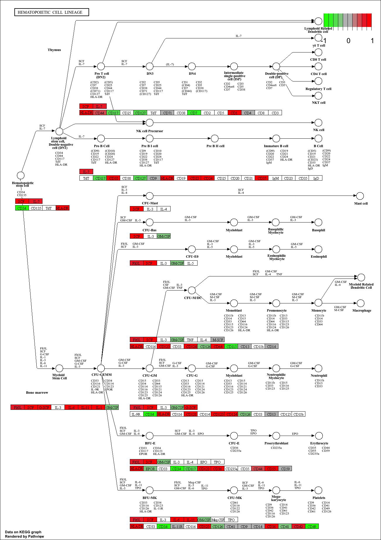
hsa04640 Hematopoietic cell lineage 0.002754415 2.854328 0.002754415
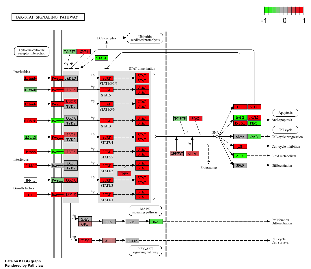
hsa04630 Jak-STAT signaling pathway 0.004331117 2.653220 0.004331117
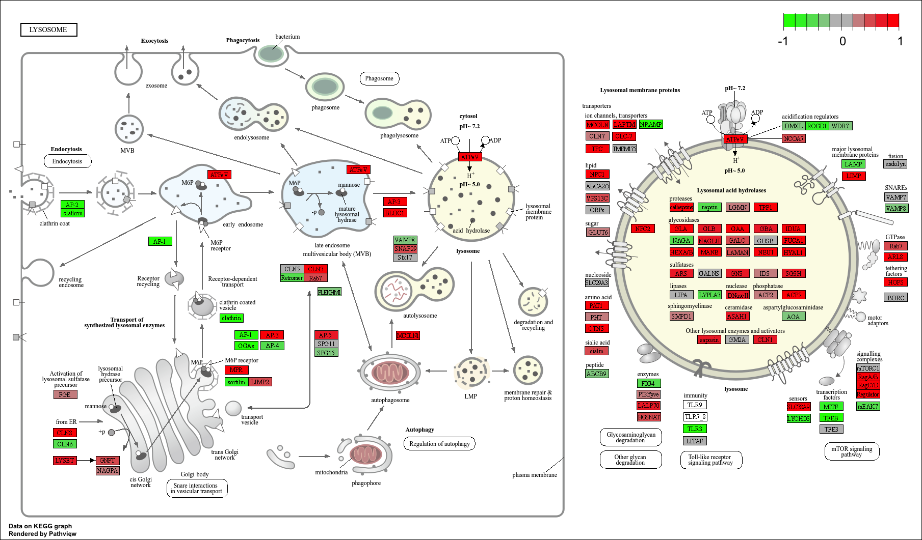
hsa04142 Lysosome 0.009214681 2.373850 0.009214681
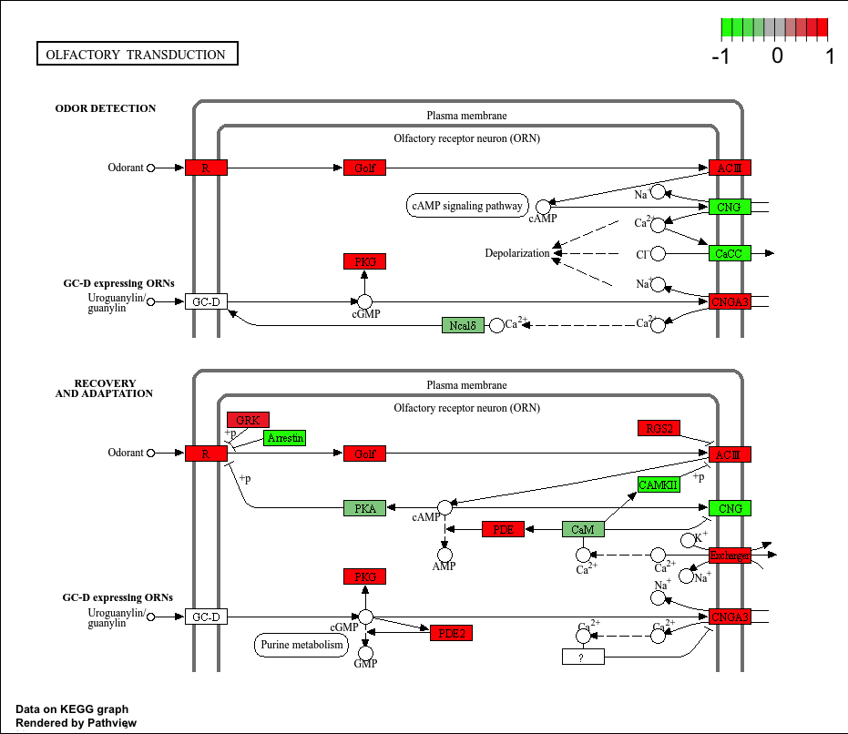
hsa04740 Olfactory transduction 0.017795693 2.158587 0.017795693
hsa04976 Bile secretion 0.025431268 1.981830 0.025431268
q.val set.size exp1
hsa00140 Steroid hormone biosynthesis 0.2203532 23 0.002628156
hsa04640 Hematopoietic cell lineage 0.2203532 48 0.002754415
hsa04630 Jak-STAT signaling pathway 0.2309929 99 0.004331117
hsa04142 Lysosome 0.3685873 116 0.009214681
hsa04740 Olfactory transduction 0.5694622 35 0.017795693
hsa04976 Bile secretion 0.5787993 42 0.025431268head(keggres$less) p.geomean stat.mean p.val
hsa04110 Cell cycle 1.195945e-05 -4.312136 1.195945e-05
hsa03030 DNA replication 9.289098e-05 -3.955346 9.289098e-05
hsa04114 Oocyte meiosis 1.245232e-03 -3.064837 1.245232e-03
hsa03013 RNA transport 2.548790e-03 -2.830112 2.548790e-03
hsa03440 Homologous recombination 3.074552e-03 -2.851878 3.074552e-03
hsa00010 Glycolysis / Gluconeogenesis 8.334721e-03 -2.439491 8.334721e-03
q.val set.size exp1
hsa04110 Cell cycle 0.001913512 120 1.195945e-05
hsa03030 DNA replication 0.007431278 36 9.289098e-05
hsa04114 Oocyte meiosis 0.066412358 98 1.245232e-03
hsa03013 RNA transport 0.098385671 142 2.548790e-03
hsa03440 Homologous recombination 0.098385671 28 3.074552e-03
hsa00010 Glycolysis / Gluconeogenesis 0.196779852 46 8.334721e-03KEGG
Top 5 upregulated KEGG pathways:
keggrespathways_up <- rownames(keggres$greater)[1:5]
keggresids_up <- substr(keggrespathways_up, start = 1, stop = 8)
keggresids_up
[1] "hsa00140" "hsa04640" "hsa04630" "hsa04142" "hsa04740"Plotting top 5 upregulated pathways:
pathview(gene.data = foldchanges, pathway.id = keggresids_up, species = "hsa")'select()' returned 1:1 mapping between keys and columnsInfo: Working in directory /Users/cyrusshabahang/Desktop/BIMM 143 Lab/bimm143_github/class14Info: Writing image file hsa00140.pathview.png'select()' returned 1:1 mapping between keys and columnsInfo: Working in directory /Users/cyrusshabahang/Desktop/BIMM 143 Lab/bimm143_github/class14Info: Writing image file hsa04640.pathview.png'select()' returned 1:1 mapping between keys and columnsInfo: Working in directory /Users/cyrusshabahang/Desktop/BIMM 143 Lab/bimm143_github/class14Info: Writing image file hsa04630.pathview.png'select()' returned 1:1 mapping between keys and columnsInfo: Working in directory /Users/cyrusshabahang/Desktop/BIMM 143 Lab/bimm143_github/class14Info: Writing image file hsa04142.pathview.png'select()' returned 1:1 mapping between keys and columnsInfo: Working in directory /Users/cyrusshabahang/Desktop/BIMM 143 Lab/bimm143_github/class14Info: Writing image file hsa04740.pathview.png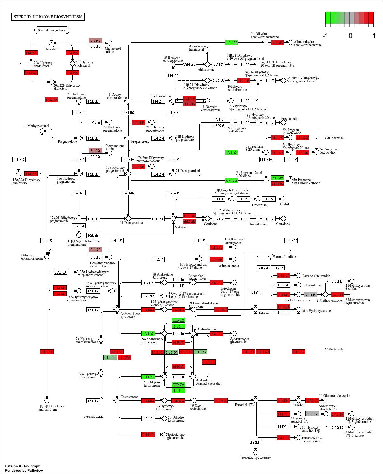
Top 5 downregulated KEGG pathways
keggrespathways_down <- rownames(keggres$less)[1:5]
keggresids_down <- substr(keggrespathways_down, start = 1, stop = 8)
keggresids_down
[1] "hsa04110" "hsa03030" "hsa04114" "hsa03013" "hsa03440"Plotting top 5 downregulated pathways:
data(go.sets.hs)
data(go.subs.hs)
Focusing on Biological Process only
gobpsets <- go.sets.hs[go.subs.hs$BP]Running gage on GO BP sets:
gobpres <- gage(foldchanges, gsets = gobpsets)Let’s view the top GO Biological Process terms:
head(gobpres$greater) #upregulated GO BP p.geomean stat.mean p.val
GO:0007156 homophilic cell adhesion 2.148684e-05 4.183707 2.148684e-05
GO:0060429 epithelium development 8.115661e-05 3.788203 8.115661e-05
GO:0048729 tissue morphogenesis 2.169820e-04 3.534688 2.169820e-04
GO:0002009 morphogenesis of an epithelium 2.337841e-04 3.518313 2.337841e-04
GO:0007610 behavior 4.656695e-04 3.324713 4.656695e-04
GO:0016337 cell-cell adhesion 5.260992e-04 3.292769 5.260992e-04
q.val set.size exp1
GO:0007156 homophilic cell adhesion 0.08403505 101 2.148684e-05
GO:0060429 epithelium development 0.15870175 459 8.115661e-05
GO:0048729 tissue morphogenesis 0.22858239 388 2.169820e-04
GO:0002009 morphogenesis of an epithelium 0.22858239 314 2.337841e-04
GO:0007610 behavior 0.34292898 380 4.656695e-04
GO:0016337 cell-cell adhesion 0.34292898 305 5.260992e-04head(gobpres$less) #downregulated GO BP p.geomean stat.mean p.val
GO:0000279 M phase 8.593273e-17 -8.395427 8.593273e-17
GO:0048285 organelle fission 7.096733e-16 -8.169833 7.096733e-16
GO:0000280 nuclear division 1.938973e-15 -8.050259 1.938973e-15
GO:0007067 mitosis 1.938973e-15 -8.050259 1.938973e-15
GO:0000087 M phase of mitotic cell cycle 5.596705e-15 -7.901860 5.596705e-15
GO:0007059 chromosome segregation 1.246925e-11 -6.966576 1.246925e-11
q.val set.size exp1
GO:0000279 M phase 3.360829e-13 484 8.593273e-17
GO:0048285 organelle fission 1.387766e-12 370 7.096733e-16
GO:0000280 nuclear division 1.895831e-12 346 1.938973e-15
GO:0007067 mitosis 1.895831e-12 346 1.938973e-15
GO:0000087 M phase of mitotic cell cycle 4.377742e-12 356 5.596705e-15
GO:0007059 chromosome segregation 8.127870e-09 139 1.246925e-11Reactome
Significant genes for Reactome upload:
sig_genes <- res[res$padj <= 0.05 & !is.na(res$padj), "symbol"]Let’s remove the missing symbols:
sig_genes <- sig_genes[!is.na(sig_genes)]
length(sig_genes)
[1] 8122Total number of significant genes is 8122.
Text file for Reactome website upload:
write.table(sig_genes,
            file = "significant_genes.txt",
            row.names = FALSE,
            col.names = FALSE,
            quote = FALSE)
Q: What pathway has the most significant “Entities p-value”? Do the most significant pathways listed match your previous KEGG results? What factors could cause differences between the two methods?
The pathway with the most significant “Entities p-value” is Cell Cycle, Mitotic with a p-value of 2.08E-5. The sginificant Reactome pathways are generally consistent with the KEGG results. The factors that could cause differences between the two methods include differences in pathway database curation and pathway definitions. Some other factors are gene id mapping and differences in background gene sets.
sig_genes <- res[res$padj <= 0.05 & !is.na(res$padj), "symbol"]
sig_genes <- sig_genes[!is.na(sig_genes)]
print(paste("Total number of significant genes:", length(sig_genes)))
[1] "Total number of significant genes: 8122"write.table(sig_genes,
file = "significant_genes.txt",
row.names = FALSE,
col.names = FALSE,
quote = FALSE)